I took part in SIGNATE's 4th AI Edge Contest, so I wanted to write up a report/log of the experience.
It wasn't just a machine learning competition — the hardware side was just as serious.
Table of Contents
1. About the network
2. C++ application code optimizations
3. About the hardware platform )
1. About the network
1.1 Model and strategy used
I used U-Net, since it's easy to customize. For libraries, I used Keras and TensorFlow, with the following versions for the conversion work prior to quantization:
・Keras==2.2.4
・tensorflow-gpu==1.13.1
I chose U-Net because it's easy to customize the network — both for going from pretrained to fine-tuned, and for tweaking the architecture to improve accuracy.
Depth was set to 512. I kept the model size relatively small so processing speed wouldn't suffer, resulting in a memory footprint of **14,067,237**.
My strategy with this model was to beat the benchmark.
The reasoning: if I could clear the benchmark this way, it would create a meaningful differentiation from other participants in terms of ingenuity and processing speed, giving me an advantage.
Model size comparison with YOLOv3
| Yolov3 | 62,002,753 |
|---|---|
| Yolov3-tyny | 8,861,918 |
| This U-Net | 14,067,237 |
Size comparison between depth 512 and depth 1024
| Depth | Size |
|---|---|
| 512 | 14,067,237 |
| 1024 | 31,055,557 |

Network diagram of the U-Net used this time
I also considered another option: using depth 1024 (memory size: 31,055,557) combined with lightweighting techniques such as pruning.
Also, since I expected this contest's segmentation task and preprocessing to increase the computational load on the hardware's PS side, I used softmax as the final layer.
Thanks to this, I was able to offload work to the softmax computation IP on the hardware side, increasing DPU utilization.
Approach I did not take
The approach I decided against was building a model with depth 1024 or greater and lightweighting it via pruning or distillation.
Techniques like pruning and distillation are heavily hardware-specific, so the learning curve and time/development cost would have been too high (especially self-taught, within the time available).
Without lightweighting, a depth-1024 model would exceed 30,000,000 parameters in memory, which directly and noticeably impacts processing speed — so I didn't go with this strategy.
1.2 Network design considerations to avoid compile-time errors
Certain layer configurations caused accuracy degradation or errors right before/after quantization, so I excluded those and built the network accordingly.
Improvements made
1. Strictly following the "Conv2D → BatchNormalization (BN) → ReLU" layer order
An invalid configuration is "ReLU → BN," which causes a compile-time error.
x = Conv2D(filters = n_filters, kernel_size = (kernel_size, kernel_size),
            kernel_initializer = 'he_normal', padding = 'same')(x)
x = BatchNormalization()(x)
x = Activation('relu')(x)
2. Using Dropout on the decoder side
Using BN on the decoder side (where Concatenate or Add layers are used) leads to accuracy degradation after quantization.
3. Using Conv2DTranspose instead of Conv2D right before softmax
Since I used softmax, in order to quantize the model I needed to use a layer other than Conv2D right before softmax (e.g., Conv2DTranspose, SeparableConv2D, etc.).
1.3 Using softmax with the DPU in mind
This time, to make use of the softmax computation IP on the hardware, I used softmax as the final layer of the U-Net as well.
Using softmax provided the following benefits:
• It allows PL, DPU computation, and softmax computation to run in parallel across three threads
• Softmax gives higher accuracy than sigmoid or ReLU
Conditions for using softmax with U-Net
Through trial and error using the DPU in Vitis, I found the following:
• As a compile-time constraint, the layer immediately before softmax must be something other than Conv2D (e.g., Conv2DTranspose, SeparableConv2D, etc.)
# Code near the final layer of the U-Net (model) during fine-tuning
x=model.get_layer(index=-5).output
x = Conv2DTranspose(nClasses, kernel_size=1, use_bias=False)(x)
x = (Activation("softmax"))(x)
• If you don't specify `use_bias=False` for Conv2DTranspose, the output of the DNNDK library's `dpuGetOutputTensorScale()` changes, which can cause errors in the softmax output
1.4 Techniques used to improve accuracy
At depth 512, simply building the network wasn't enough to exceed IoU=60% — I needed accuracy-improvement techniques beyond just the network architecture itself.
Here are the main techniques I used.
Resizing that preserves the original image's (height, width) aspect ratio
=> I resized to shape (400, 680), preserving the original image's size ratio, and used OpenCV's resize while maintaining the aspect ratio. This improved prediction accuracy for small objects (signals, pedestrians) compared to resizing to a square shape like (224, 224).
I think this is because it reduced the loss of positional information during resizing.
Preprocessing to brighten dark images (mean pixel value below 80) via histogram equalization
=> This slightly improved accuracy for fine details in dark images. Since dark images tend to have skewed pixel distributions, I treated
"low mean pixel value = dark image"
and applied histogram equalization to images with a mean pixel value under 80 to brighten them.
def clahe(bgr):
    #plt.imshow(bgr),plt.show()
    lab = cv2.cvtColor(bgr, cv2.COLOR_BGR2LAB)
    #plt.imshow(lab),plt.show()
    lab_planes = cv2.split(lab)
    clahe = cv2.createCLAHE(clipLimit=6.0,tileGridSize=(8,8))
    lab_planes[0] = clahe.apply(lab_planes[0])
    lab = cv2.merge(lab_planes)
    return cv2.cvtColor(lab, cv2.COLOR_LAB2BGR)

def NormalizeImageArr(path, H, W):
    NORM_FACTOR = 255
    img = cv2.imread(path, 1)
    img = cv2.resize(img, (H, W), interpolation=cv2.INTER_NEAREST)
    if img.mean()<80:
        img = clahe(img)
    img = img.astype(np.float32)
    img = img/NORM_FACTOR
    return img
Training with augmentation
Augmentations that didn't change object position (noise, contrast adjustments, horizontal flip) were the most effective.
Vertical flip backfired when objects (like cars) never appear upside down.
Also, rather than applying all augmentations at once, gradually introducing them step by step seemed to steadily improve accuracy.
I trained with augmentation using the following steps:
| Epoch | Dataset | IOU | Augmentation |
|---|---|---|---|
| 100 | CitySpacuies | None | None |
| 200 | train: 2,143 images (contest images), val: 100 images (contest images) | train=83.8%、Val = 74% | None |
| 200 | train: 2,143 images (flipped only), val: 100 images (flipped only) | train=76%、Val = 68% | Horizontal flip (also applied to validation) |
| 100 | train:4286 images、val:100 images | train=88.5%、Val = 75.8% | Horizontal flip (not applied to val) |
| 100 | train:4286 images、val:100 images | train=89.2%、Val = 77.5% | contrast-based(not applied to val) |
Pretraining on the Cityscapes dataset
I borrowed this idea from a precedent set in a previous contest, and it improved accuracy considerably.
I also tried adding residual structures and sub-layers favorable for segmentation, but at depth 512 the model's representational capacity had reached its limit, so this had almost no effect. It was also tough that layers like SENet (which use multiply operations) ran into compile-time errors, which was a hard constraint that prevented further accuracy improvements in that direction.
What I learned through this PDCA process is that applying techniques haphazardly, without some hypothesis or logic for why they should improve accuracy, mostly ends up being wasted effort.
1.5 Final network results (IoU, etc.)
In the end, with a model size of 14,067,237, I achieved an IoU of roughly 61%.
2. C++ application code optimizations
To maximize processing speed and squeeze out hardware performance, I focused especially on two things in C++.
2.1 Reducing computational load
Since the PS-side computation was heavy this time, and I used three threads, cutting down and simplifying redundant code had a meaningful effect on processing speed.
In particular, the following kinds of rewrites sped things up by roughly 30ms per improvement:
・Making `for` loops more efficient
・Removing unnecessary functions and unnecessary calls to those functions
・Turning fixed values into constants
2.2. Three-way multithreading to draw out hardware performance
Since this contest involved a lot of PS-side computation outside of the DPU (e.g., preprocessing and `for` loops for segmentation), splitting the work across three threads sped things up by roughly 30–50ms.
Below is the difference in speed between two threads and three threads, under DPU parameters (B1152, "DSP48 USAGE=LOW", etc.):
| Number of threads | Average processing time per image (ms) |
|---|---|
| 2 | 1061 |
| 3 | 1007 |
2.3 Further speed improvement by running PS, PL (DPU computation), and softmax computation in parallel across three threads
The original purpose of multithreading is to speed things up by running PS and PL in parallel. However, since I was using the DNNDK library this time, PL work is split into two independent methods:
• DPU computation
• Softmax computation
| DPU computation method | dpuRunTask() |
|---|---|
| Softmax computation method | dpuRunSoftmax() |
Because of this, I made the following three things the targets of parallel multithreaded processing:
・ DPU computation
・ Softmax computatio
By applying asynchronous processing std::lock_guard lock(mtx_) to both the DPU computation and softmax computation, I was able to run DPU computation and softmax computation in parallel, achieving a further speed improvement through multithreading.
Excerpt of the multithreaded function (main_thread()) that runs PS, DPU computation (PL), and softmax computation (PL) in parallel (key sections only)
#include <thread>
#include <opencv2/opencv.hpp>
#include <opencv2/core.hpp>
#include <dnndk/dnndk.h>
#include <mutex>
std::mutex mtx_;
〜〜
〜〜

int main_thread(DPUKernel *kernelConv, int s_num, int e_num, int tid){
  assert(kernelConv);
  DPUTask *task = dpuCreateTask(kernelConv, DPU_MODE_NORMAL);
  〜〜〜
  // Main Loop
  int cnt=0;
  for(cnt=s_num; cnt<=e_num; cnt+=BLOCK_SIZE){
      for(int i=0; i<BLOCK_SIZE;i++){
        if(cnt+i>e_num) break;
        Mat img;
        resize(input_image[i], img, for_resize, INTER_NEAREST);
        // pre-process with histgram avaraving
        Mat clahe_img = img;
        if((int)mean(img)[0] < 80) {
           clahe_img = clahe_preprocess(img);
        }

        float *softmax = new float[outWidth*outHeight*outChannel]
        // Set image into Conv Task with mean value
        set_input_image(task, outWidth, clahe_img);
        {
          std::lock_guard<std::mutex> lock(mtx_);
          dpuRunTask(task);
        }
        {
          std::lock_guard<std::mutex> lock(mtx_);
          //cout << "outScale : " << outScale << endl;
          int8_t *outAddr = (int8_t *)dpuGetOutputTensorAddress(task, CONV_OUTPUT_NODE);
          dpuRunSoftmax(outAddr, softmax, outChannel,outSize/outChannel, outScale);
        }

        // Post process
        PostProc(softmax, outHeight, outWidth, outChannel, image_file_name[i].c_str());
        delete[] softmax;
      }
  }
  dpuDestroyTask(task);
   return 0;
}

Three threads running PS, DPU computation, and softmax computation in parallel
3. About the hardware platform
3.1 Development environment
I referred to a Vitis-AI development environment article on Qiita. I didn't use the Vitis-AI-Runtime library, and instead built on top of the DNNDK library.
3.2 Notes on building the DPU hardware platform
I mainly referred to the Vitis-AI environment setup tutorial and materials from the 2nd AI Edge Contest (referred to below as "reference materials"), and built the platform by improving on the tutorial's platform.
3.2.1 Making use of the softmax computation IP
To make the most of DPU computation, I made use of the softmax computation IP.
Since I used Conv2DTranspose in the U-Net, and designed the model with this integration in mind, I used softmax computation.
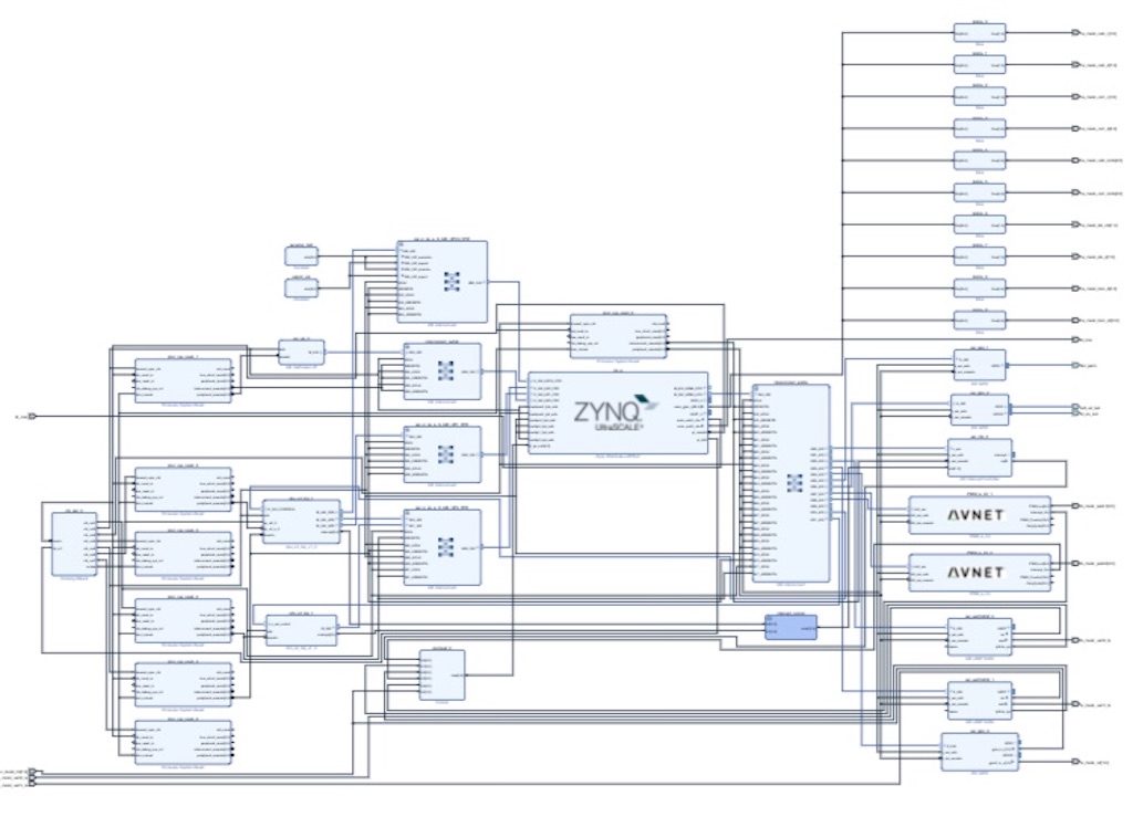
Platform including softmax computation (unnecessary IPs already removed)
3.2.2 Building and refining the platform
Since development was based on DNNDK, I mainly refined the Vitis-AI platform tutorial, using the reference materials as a guide.
Initially, my first goal was to get a platform with a DPU installed working under the following conditions from the reference materials:
•DPU frequency of 250MHz
To do this, I first took the tutorial's platform and:
2. Removed unnecessary clocks
and built the platform with WNS = 0.027 .
This time, because I needed to enable "DepthwiseConv" in order to use my model, I had to make changes to the parameters and frequency.
3.3 DPU parameters and frequency
That change made the parameter set too large — pushing the frequency higher caused the board to reboot, so I couldn’t get a DPU running with B1600 at 250MHz
On top of that, since “DepthwiseConv” uses 3,292 LUTs on B1600, I had to significantly reduce the DPU parameter resources compared to the reference materials.
In particular, since this model makes heavy use of convolutional layers, without enabling "Channel Augmentation," processing speed dropped considerably even with "DSP48 Usage" set to High. So I made the following mandatory:
・Enable "DepthWiseConv"
As a result, at frequencies of 225MHz or higher with "DSP48 USAGE" set to HIGH, the board would reboot. So in the end, I settled on a frequency of 200MHz with the following parameters for the DPU:
| Frequency | 200MHz |
|---|---|
| DPU | B1600(ReLU+ReLU6) |
| Channel Augmentation | Enable |
| DepthWiseConv | Enable |
| PoolAverage | Disnable |
| DSP48 USAGE | HIGH |
| RAM USAGE | LOW |
| Softmax | Enable |
Given the resource constraints, I wasn't able to push the frequency any higher than this.
3.4 Improving processing speed via impl and synth strategies
At 200MHz with this DPU parameter set, the frequency alone wasn't enough to draw out the DPU's full performance. So I tried several strategy combinations to see if I could improve processing speed further, referring to an article from Fixstars' site.
According to the "High-Density FPGA Design Guide", the more resources you use, the lower the integration density needs to be in order to make effective use of those resources.
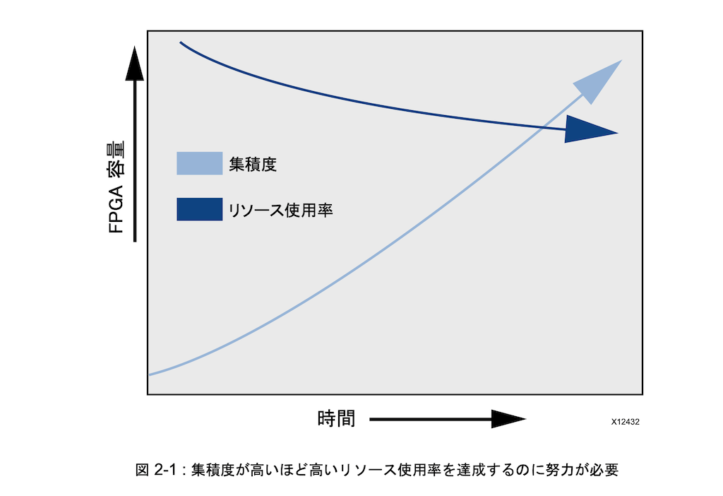
Since the DPU had a lot of resources allocated this time, I chose a combination of strategies that spread the logic out to lower the integration density — this sped things up by about 35ms:
| impl | Congestion_SpreadLogic_high |
|---|---|
| Synth | Flow_AreaOptimized_high |
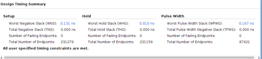
| WNS | 0.131 ns |
I also tried the SSI-distributing strategy "impl: Congestion_SSI_SpreadLogic_low." While SSI has lower power consumption, its integration density is higher, so the combination above gave better processing performance.
With this strategy combination, B1600, and a 200MHz frequency, I was able to fit a DPU that satisfied all the constraints.
Compared to PS, the utilization of DPU and softmax ended up as follows:
| PS & PL Tototal | 93% |
|---|---|
| DPU | 43% |
| Softmax | 6% |

Power consumption report for this build
References
・vitis-AI platform site(qiita)
・Xilinx GitHub Vitis-AI-TUTORIAL
・Trying different Vivado synthesis/implementation strategies(WNS & runtime)